1. Data Processing

In order to know what kind of publicity expenses matters more in determining the profit of a company and what the relation would be, we collect the data from 50 different companies in 3 different cities about their expenses on print media, social media and outdoor advertisement. Based on this data, we could build a model to analyze the relationship.

1.1 Raw Data

Print Media Expenses	Social Media Expenses	Outdoor Ad Expenses	City	Profit
165349.2	136897.8	471784.1	Mumbai	192261.8
162597.7	151377.6	443898.5	Chandigarh	191792.1
153441.5	101145.6	407934.5	Delhi	191050.4
144372.4	118671.9	383199.6	Mumbai	182902
142107.3	91391.77	366168.4	Delhi	166187.9
131876.9	99814.71	362861.4	Mumbai	156991.1
134615.5	147198.9	127716.8	Chandigarh	156122.5
130298.1	145530.1	323876.7	Delhi	155752.6
120542.5	148719	311613.3	Mumbai	152211.8
123334.9	108679.2	304981.6	Chandigarh	149760
101913.1	110594.1	229161	Delhi	146122
100672	91790.61	249744.6	Chandigarh	144259.4
93863.75	127320.4	249839.4	Delhi	141585.5
91992.39	135495.1	252664.9	Chandigarh	134307.4
119943.2	156547.4	256512.9	Delhi	132602.7
114523.6	122616.8	261776.2	Mumbai	129917
78013.11	121597.6	264346.1	Chandigarh	126992.9
94657.16	145077.6	282574.3	Mumbai	125370.4
91749.16	114175.8	294919.6	Delhi	124266.9
86419.7	153514.1	0	Mumbai	122776.9
76253.86	113867.3	298664.5	Chandigarh	118474
78389.47	153773.4	299737.3	Mumbai	111313
73994.56	122782.8	303319.3	Delhi	110352.3
67532.53	105751	304768.7	Delhi	108734
77044.01	99281.34	140574.8	Mumbai	108552
64664.71	139553.2	137962.6	Chandigarh	107404.3
75328.87	144136	134050.1	Delhi	105733.5
72107.6	127864.6	353183.8	Mumbai	105008.3
66051.52	182645.6	118148.2	Delhi	103282.4
65605.48	153032.1	107138.4	Mumbai	101004.6
61994.48	115641.3	91131.24	Delhi	99937.59
61136.38	152701.9	88218.23	Mumbai	97483.56
63408.86	129219.6	46085.25	Chandigarh	97427.84
55493.95	103057.5	214634.8	Delhi	96778.92
46426.07	157693.9	210797.7	Chandigarh	96712.8
46014.02	85047.44	205517.6	Mumbai	96479.51
28663.76	127056.2	201126.8	Delhi	90708.19
44069.95	51283.14	197029.4	Chandigarh	89949.14
20229.59	65947.93	185265.1	Mumbai	81229.06
38558.51	82982.09	174999.3	Chandigarh	81005.76
28754.33	118546.1	172795.7	Chandigarh	78239.91
27892.92	84710.77	164470.7	Delhi	77798.83
23640.93	96189.63	148001.1	Chandigarh	71498.49
15505.73	127382.3	35534.17	Mumbai	69758.98
22177.74	154806.1	28334.72	Chandigarh	65200.33
1000.23	124153	1903.93	Mumbai	64926.08
1315.46	115816.2	297114.5	Delhi	49490.75
0	135426.9	0	Chandigarh	42559.73
542.05	51743.15	0	Mumbai	35673.41
0	116983.8	45173.06	Chandigarh	14681.4

The raw data is shown above.

1.2 Drop Zero Data

Drop all data with null values in the table to prevent extreme outliers.

1.3 Categorical Variable

Column “City” contains labels, Mumbai, Chandigah and Delhi, which cannot be used for linear regression. Thus, transform them into dummy variables.

Because there are three different cities, two dummy variables $z_1$ and $z_2$ are needed.

As the table below shows, (0, 1) represents Munbai, (1, 0) represents Chandigah, and (0, 0) represents Delhi.

	$z_1$	$z_2$
Mumbai	0	1
Chandigah	1	0
Delhi	0	0

1.4 Data Description

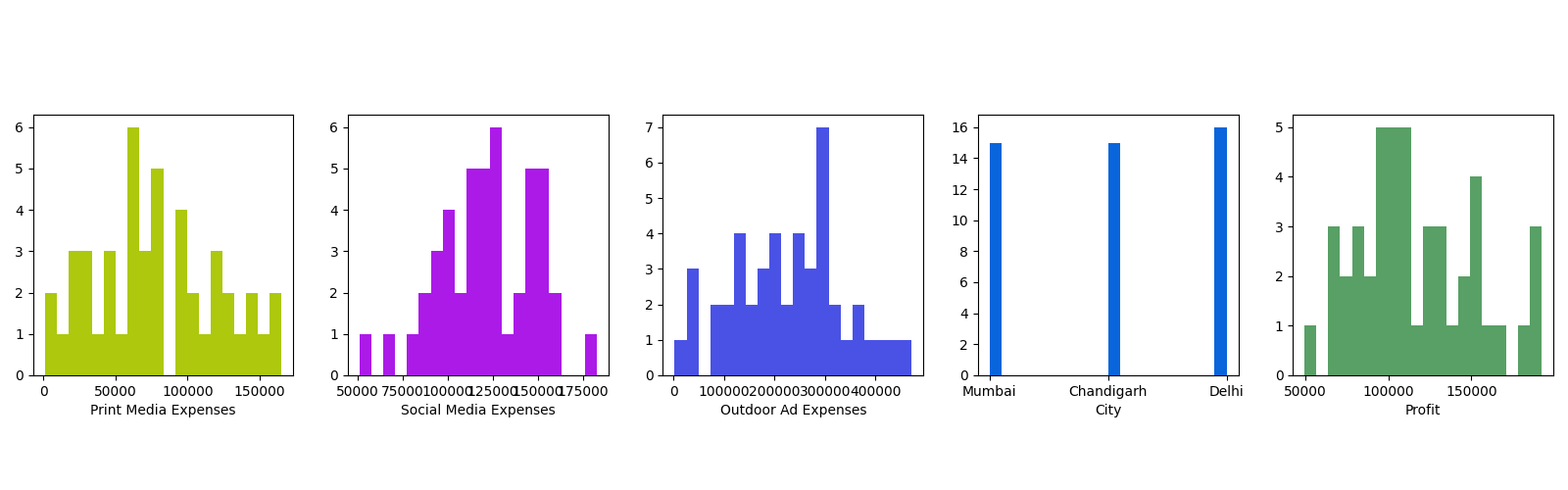
Based on these simply processed data, the following figures are drawn. In the data, the spendings of all 46 companies on three different advertising methods are counted.

For print media expenses and social media expenses, the overall spending level is low, basically below 200,000, mostly concentrating between 50,000 and 150,000. In outdoor advertising expenses, most companies invest more than 100,000, among which the highest reaches 450,000.

For print and social media expenses, up to 6 sets of data locates in the same range, and for outdoor advertising spending, up to 7 sets. Regarding cities of the companies, Mumbai and Chandigah each accounts for 15, and Delhi 16.

For profit of the companies, it is distributed in the range of 50,000 to 200,000. Most of the companies have a profit around 100,000. There is only one company with a profit of 50000, and four companies with a profit of 200000, accounting for a very small proportion.

2. Data Test

In order to use multiple linear regression to build our model, several conditions must be satisfied. Therefore, we use several tests to check out whether the independent variables are good candidates for multiple linear regression.

2.1 Linear Relationship between Independent Variables and Dependent Variable

2.1.1 Scatter Plot

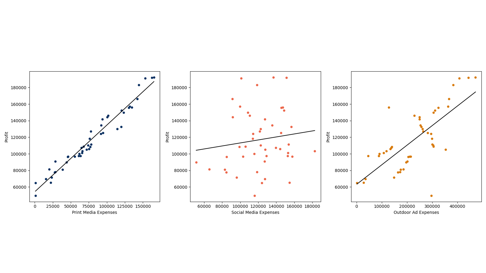
Three figures below show the value of profit versus three different expenses.

Fig 2.1 and 2.3 shows a strong linear relationship between profit and print media expenses and outdoor ad expenses. Fig 2.2 shows the weak linear relationships between profit and social media expenses.

2.1.2 Correlation Coefficient

To better analyze the linear relationship between profit and expenses, we compute the correlation coefficients, which is shown above.

The table shows strong linear relationships between $y$ and $x_1, x_3$. But, the relationship between $y$ and $x_2$ is weak, so as $z_1$ and $z_2$. However, $z_1$ and $z_2$ are categorical variables, which just has values of 0 or 1. Therefore, generally profit has linear relationship with expenses.

	$x_1$	$x_2$	$x_3$	$z_1$	$z_2$
$y$	0.97	0.13	0.73	-0.06	0.03

2.2 Independence between Variables

2.2.1 Residual Plot

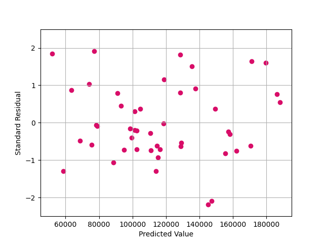
In the residual plot we could see that the data points show no significant trend along x **or y axis.

Regarding the source, the data comes from different companies in 3 different cities, which leads to low interaction between these companies. Together with the residual plot shown above, we roughly consider our variables to be independent.

2.3 Normality for Residuals

2.3.1 Q-Q Plot

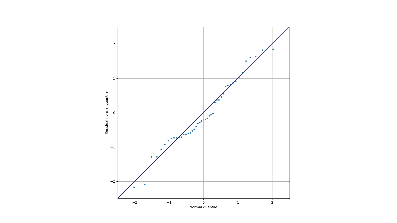
To roughly see whether the residuals follow normal distribution, we scatch the quantile-quantile plot, which is shown below.

In the figure, we could see that the scatter points lie close to the marked straight line, which means that the distribution of these residuals are approximately normal.

2.3.2 Kolmogorov–Smirnov Test

Normality of data is of very high importance in our regression, so we do further K-S test to confirm it.

With our data and following equations, we compute $D_n$, the K-S statistic of our data to be 0.1153. Referring the table, we know that the limit for our data to be normal is 0.1698, which is significantly higher than 0.1153. Therefore, we could consider that our data follows normal distribution.

$$r_i=y_i-\hat y_i$$ $$F_{exp}(r_i)=\frac{i}{n}, i=1,2, \dots,n$$ $$F_{obs}(r_i)=P(z\lt\frac{r_i-\mu}{\sigma})$$ $$D_n=max(|F_{exp}(r_i)-F_{obs}(r_i)|),r_1\le r_2\le\cdots\le r_n$$ $$D_n=0.1153<D_c=0.1698$$

2.4 Equal Variance

2.4.1 Residual - Predicted Value Plot

To build our multiple linear regression model, equal variance is also a very important need. So, we use the residual plot to see if there is an obvious trend of residuals regarding the change of profit. As Fig 5, the residuals seem random and homogeneous around zero, without significant increasing, decreasing or bending. Therefore, we consider our model to be with equal variance.

3. Data Regression

3.1 Multicollinearity

3.1.1 Correlation Matrix

	$x_1$	$x_2$	$x_3$	$z_1$	$z_2$
$x_1$	1	0.2	0.71	-0.08	0.04
$x_2$	0.2	1	-0.09	-0.05	0.06
$x_3$	0.71	-0.09	1	-0.15	0.03
$z_1$	-0.08	-0.05	-0.15	1 ng	-0.48
$z_2$	0.04	0.06	0.03	-0.48	1

To build our regression model, we must ensure that multicollinearity is not severe between all these variables, which means that no two variables share highly similar linear relationship between profit and itself.

So, we construct the correlation matrix, which is shown in the above table. As all these computations show, most of their correlation coefficients are much smaller than 0.7. Therefore, our model shows low multicollinearity.

3.1.1 Analysis of Eigenvalues

For matrix $X'X$, all the eigenvalues are shown above. With all the computations of k, the maximum one gives the value of 7.77, which is smaller than 100. Therefore, we could consider our variables to have very low level of multicollinearity and thus could be used in analysis.

$$X=\begin{bmatrix}x_{11}&x_{21}&\cdots&x_{51}\\x_{12}&x_{22}&\cdots&x_{52}\\\vdots&\vdots&\vdots&\vdots\\x_{1n}&x_{2n}&\cdots&x_{5n}\end{bmatrix}$$ $$A=X'X$$ $$\lambda_1=82.85,\lambda_2=10.66,\lambda_3=23.68,\lambda_4=65.01,\lambda_5=47.81$$ $$k=\frac{\lambda_1}{\lambda_2}=7.77\lt100$$

3.2 Regression

3.2.1 Forward Selection

Step 1:

$$R^2=1-\frac{SSE}{SST}$$

	$\hat y$	$R^2$	$f$
$x_1$	$\hat y=54110+0.8046x_1$	0.95585	952.60249
$x_2$	$\hat y=94970+0.1812x_2$	0.01825
$x_3$	$\hat y=63050+0.2365x_3$	0.53617

From the $R^2$ we get, we could find that $R^2_1$ > $R^2_2$ > $R^2_3$, and the largest $R^2$ is from $x_1$. Then we will take F-test of $x_1$. And according to the table of F-test, we could find that f = 952.60249 > $f_{0.05}(k-1,n-k-1)$, so $x_1$ is significant, and we choose $x_1$. Then the procedure will continue and we will insert a new variable.

Step 2:

$$R(\beta_i|\beta_j)=R(\beta_i,\beta_j)-R(\beta_i)$$ $$f=\frac{SSR/(k-1)}{SSE/(n-k-1)}$$

	$\hat y$	$R(\beta_i, \beta_1)$	$f$
$x_1,x_2$	$\hat y=63000+0.8141x_1-0.07897x_2$	193839556	3.51402
$x_1,x_3$	$\hat y=51860+0.7581x_1+0.02580x_3$	193319026

$f_{0.05}(k-1, n-k-1) > 3.51402$

Therefore, adding more variables doesn’t give a significant change to the model. So the procedure is terminated.

Then we find only $x_1$ gives a significant change to this model, as a result, we could get:

$\hat y=54110+0.8046x_1$

That means: $Profit = 54110 + 0.8046 \times Print Media Expenses$

3.2.2 Backward Elimination

Step 1: Fit all the variables

	$\beta$	$R^2$	$f$
$x_1$	0.806	0.951	295.978
$x_2$	-0.027
$x_3$	0.027

Step 2: Remove x2

	$\beta$	$R^2$	$f$
$x_1$	0.797	0.950	450.771
$x_3$	0.030

Step 3: Remove x3

$$\hat y=54110+0.8046x_1$$

	$\beta$	$R^2$	$f$
$x_1$	0.854	0.947	849.789

Backward Elimination analysis was performed with Print Media Expenses, Social Media Expenses, and Outdoor Ad Expenses as independent variables, and Profit as the dependent variable. After calculation, only Print Media Expenses have the significant change to this model.

$Profit=54110+0.8046x_1\times PrintMediaExpenses$

4. Hypotheses Testing

4.1 Effects of Different Kinds of Expenses

We are firstly interested in whether one certain expense impacts profit significantly under the condition that other expenses are put. So we use the model containing all the variables to do the hypotheses testing.

$$\begin{aligned}H_0&:\beta_j=\beta_{j0}\\H_1&:\beta_j\ne \beta_{j0}\end{aligned}$$ $$t=\frac{\hat\beta_j-\beta_{j0}}{s\sqrt{c_{jj}}}$$ $$\hat\beta_j-t_{\alpha/2}\cdot s\sqrt{c_{jj}}\lt\beta_j\lt\hat\beta_j+t_{\alpha/2}\cdot s\sqrt{c_{jj}}$$

In the test, the t values for the critical region are -2.021 and 2.021.

For $\beta_1$, we use the data to compute the corresponding $t$-statistic to be 19.8, which exceeds the $t$-statistic for the critical region.

Similarly, for $\beta_2$ and $\beta_3$, the corresponding $t$-statistics are about -1.28 and 1.38, which are smaller than the corresponding t-statistic for the critical region.

Therefore, we can reject the null hypothesis for $\beta_1$ but not for $\beta_2$ and $\beta_3$, which means we can not reject $\beta_2$ or $\beta_3$ to be 0 in the presense of the other two.

That is to say, except print media expenses, one certain expense have insignificant impact on the profit under the existence of the other two expenses. Thus, print media expense may be the most important one in the three expenses.

4.2 Effects of Different Cities

4.2.1 One-Way ANOVA

We are then interested in whether the cities of these companies have a significant impact on their profit. So, we continue to construct our hypotheses-testing process.

$$\begin{aligned}H_0&:\mu_1=\mu_2=\mu_3\\H_1&:any\ of\ them\ is\ different\end{aligned}$$ $$f=0.0790\lt f_{0.05}(2,42)$$ $$\therefore can\ not\ reject\ H_0$$

We first set our null hypothesis to be that the means of profit for companies in these three cities are equal. Then, the alternative hypothesis is that any of these two means are not equal.

For only one single factor is considered there, we use One-Way ANOVA to test our hypothesis and the results are shown above. The treatment sum of squares SSA, with degrees of freedom to be 2, has its mean square about 109051702.16. And the error sum of squares SSE, with degrees of freedom to be 42, has mean square about 1380294796.39.

So, the f-statistic computed is 0.0790, which is much smaller than the f-statistic for the critical region. Therefore, we can not reject our null hypothesis. Thus, we could get the conclusion that we can not reject the profit of all the companies in three cities share the same mean value.

That is to say, the impact of cities on the profit a company make is insignificant.

Source	DF	SS	MS	f
SSA	2	218103404.31	109051702.16	0.0790
SSE	42	57972381448.24	1380294796.39
SST	44	58190484852.56

5. Conclusion

From all the processes above, we could get the conclusion that the print media expense matters most in determining the profit, followed by outdoor ad expense and then social media expense. What’s more, the effect of city is insignificant.

For all the models we build, $R^2_{adj}$ is computed to be larger than 0.95, which means that most of the observed values of profit could be explained by the model. Besides, the MAPE (Mean Absolute Percentage Error) is computed to be lower than 1%.

Additionally, the linearity between response and responsors, the normality and equal variance are all significant.

Therefore, we eveluate our regression models to be good ones.

However, shortcomings still exist.

First, the number of companies in each city is not very large. Thus, the data may not support the results very strongly.

Second, we can not confirm our variables to be of high level of independence.

Third, the multicollinearity between print media expenses and outdoor ad expenses is not very low, which may disturb the regression results.

Fourth, we can not confirm these 46 companies to have similar conditions and other expenses, without which the regression results would be inaccurate.

Therefore, if further improvements are to be conducted, ways might be found through the above four points.

6. Contributions

Team Member	Contributions
Ke Xu	Planning the structure; programming and coding; data searching, processing and testing; regression; hypotheses testing; writing report; making slides.
Yifan Chen	Planning the structure; coding; data searching, description and testing; regression; hypotheses testing; writing report; making slides.
Ruiwen Zhang	Forward selection; writing report.
Zeyi Yang	Backward elimination; writing report.
Zhuo Wang	Data description; writing report.